Single-Variant Precision Analysis

Nicholas Mikolajewicz

2020-05-28

Single-Variant Precision Analyses

Single-variant precision (SVP) analyses aim to calculate the inherent variability of an instrument, without consideration for time- or scanner-dependent sources of error. That is, precision estimates are calculated by first computing replicate-level statistics (e.g., triplicate phantom scans at a single time point by a single scanner), and then pooled across all scanners and time points to yield a root-mean-square (RMS)- or median-based precision estimate. This is commonly known as a short-term single-scanner/site precision estimate and conveys how precise/reproducible a given technology is at a given point in time, without consideration for external factors, such as drift over time, or between-scanner discrepancies.

Data import and prep

Prior to analysis, import data and preprocess as described in the Getting Started Vignette.

# import data
input.data <- efp

# create Calibration Object
co <- createCalibrationObject(input.data)

# get list of feature subsets to analyze
analyze.these <- analyzeWhich(co,
                              include.sections = seq(1,3),
                              include.parameters = c("Tb.vBMD", "Tt.vBMD", "Tb.BVTV", "Ct.vBMD.XCTII", "Ct.Th.XCTII"),
                              omit.parameters = c("Tb. BVTV"))

# preprocess/filter data
co <- preprocessData(object = co,
                      analyze.which = analyze.these,
                      new.assay.name = "preprocessed.data",
                      which.assay = "input")

SVP Analysis

Lets calculate short-term single-site precision errors for our uncalibrated data stored in the preprocessed Assay using svpAnalysis.

# calculate short-term precision errors for uncalibrated data
co <- svpAnalysis(co,
                   which.data = "uncalibrated",
                   verbose = F)

Tip: Since the svpAnalysis contains an “Analysis” suffix, results are stored in the analysis slot of the current Assay. This pattern of assignment within the Calibration Object is consistent throughout the XcalRep Package.

svpAnalysis generates two sets of tables which can be retrieved from the Calibration Object using getResults. The replicate.statistics table reports descriptive statistics for replicate scans and the rms.statistics table reports root-mean-square (RMS) statistics (i.e., short-term single-site precision error estimates). Note that median-based statistics are also provided in the rms.statistics results table, and can provide robust estimates of precision in the presence of outliers. .

Let’s take a look at the root-mean-square statistics.

# retrieve stored results (as datatables)
svp.results.uncalibrated <-getResults(object = co,
                                which.results = "svp",
                                format = 'dt') # 'dt' (datatable) or 'df' (dataframe)

#> Warning in getResults(object = co, which.results = "svp", format = "dt"):
#> returning results for 'uncalibrated' dataset

# see what tables were generated 
names(svp.results.uncalibrated)

#> [1] "replicate.statistics"       "rms.statistics"            
#> [3] "rms.statistics.no.outliers"

# show rms statistics
showTable(svp.results.uncalibrated[["rms.statistics"]])

Outliers

Outliers are automatically flagged during SVP analysis and two sets of rms statistics tables are generated; rms.statistics contains statistics computed using all data, and rms.statistics.no.outliers contains results where outliers were omitted. Additionally, the replicate.statistics table contains an outlier.flag feature which flags suspected outliers. While it is generally poor practice to omit outiers from precision analyses, in the context of a multi-centre trial it may be informative to identify outlying sites. If outliers appear randomly distributed throughout the dataset and there is not discernable bias (e.g., all outlying data comes from a single site), it is recommended to retain all data for downstream analysis. If outlier prevalence is biased towards a certain site, users should investigate the source of error further.

The easiest way to appraise outliers is to examine the replicate.statistics interactive datatable and sort entries using outlier.flag.

# show replicate statistics
showTable(svp.results.uncalibrated[["replicate.statistics"]])

Tip: The showTable function provides users with an easy way to generate tables as interactive data tables (as seen above) or as data frames. Interactive data tables allow users to export results directy into their clipboard or to csv or excel, and enable easy data filtering, sorting and exploration in the R Studio Enviroment.

Visualize Results

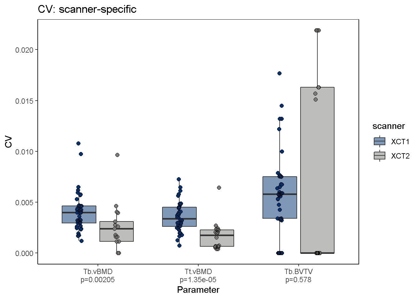
To visualize svpAnalysis results, use the svpPlot function. The default output plots CV-based precision errors, however STD-based precision errors can also be plotted using the var2plot argument. In this example we omit outliers and stratify the data by HR-pQCT scanner to determine whether 2nd generation XtremeCT scanners (XCT2) are more precise than 1st generation scanners (XCT1).

Kruskal-Wallis rank sum test is also performed (using group.by argument for data stratification) and p-values are shown for each comparison group. Significant differences in precision errors are observed between XCT and XCT2 scanners.

svpPlot(co,
         which.data = "uncalibrated",
         group.by = "scanner",
         outliers = F,
         color.begin = 0.1, color.end = 0.5)

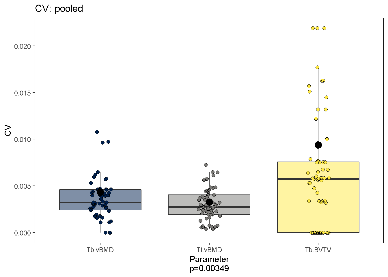
We can also ask which parameters are most reproducible; The current dataset suggests that Ct. vBMD and Tt. vBMD measures are.

svpPlot(co,
         which.data = "uncalibrated",
          outliers = F)